Fit and select bivariate copula models

Fit a bivariate copula model for continuous or discrete data. The family can be selected automatically from a vector of options.

bicop(
  data,
  var_types = c("c", "c"),
  family_set = "all",
  par_method = "mle",
  nonpar_method = "quadratic",
  mult = 1,
  selcrit = "aic",
  weights = numeric(),
  psi0 = 0.9,
  presel = TRUE,
  keep_data = FALSE,
  cores = 1
)

Arguments

data: a matrix or data.frame with at least two columns, containing the (pseudo-)observations for the two variables (copula data should have approximately uniform margins). More columns are required for discrete models, see Details.
var_types: variable types, a length 2 vector; e.g., c("c", "c") for both continuous (default), or c("c", "d") for first variable continuous and second discrete.
family_set: a character vector of families; see Details for additional options.
par_method: the estimation method for parametric models, either "mle" for maximum likelihood or "itau" for inversion of Kendall's tau (only available for one-parameter families and "t".
nonpar_method: the estimation method for nonparametric models, either "constant" for the standard transformation estimator, or "linear"/"quadratic" for the local-likelihood approximations of order one/two.
mult: multiplier for the smoothing parameters of nonparametric families. Values larger than 1 make the estimate more smooth, values less than 1 less smooth.
selcrit: criterion for family selection, either "loglik", "aic", "bic", "mbic". For vinecop() there is the additional option "mbicv".
weights: optional vector of weights for each observation.
psi0: see mBICV().
presel: whether the family set should be thinned out according to symmetry characteristics of the data.
keep_data: whether the data should be stored (necessary for using fitted()).
cores: number of cores to use; if more than 1, estimation for multiple families is done in parallel.

Value

An object inheriting from classes bicop and bicop_dist . In addition to the entries contained in bicop_dist(), objects from the bicop class contain:

data (optionally, if keep_data = TRUE was used), the dataset that was passed to bicop().
controls, a list with the set of fit controls that was passed to bicop().
loglik the log-likelihood.
nobs, an integer with the number of observations that was used to fit the model.

Details

If there are missing data (i.e., NA entries), incomplete observations are discarded before fitting the copula.

Discrete variables

When at least one variable is discrete, more than two columns are required for data: the first \(n \times 2\) block contains realizations of \(F_{X_1}(x_1), F_{X_2}(x_2)\). The second \(n \times 2\) block contains realizations of \(F_{X_1}(x_1^-), F_{X_1}(x_1^-)\). The minus indicates a left-sided limit of the cdf. For, e.g., an integer-valued variable, it holds \(F_{X_1}(x_1^-) = F_{X_1}(x_1 - 1)\). For continuous variables the left limit and the cdf itself coincide. Respective columns can be omitted in the second block.

Family collections

The family_set argument accepts all families in bicop_dist() plus the following convenience definitions:

"all" contains all the families,
"parametric" contains the parametric families (all except "tll"),
"nonparametric" contains the nonparametric families ("indep" and "tll")
"onepar" contains the parametric families with a single parameter,

("gaussian", "clayton", "gumbel", "frank", and "joe"),

"twopar" contains the parametric families with two parameters ("t", "bb1", "bb6", "bb7", and "bb8"),
"elliptical" contains the elliptical families,
"archimedean" contains the archimedean families,
"BB" contains the BB families,
"itau" families for which estimation by Kendall's tau inversion is available ("indep","gaussian", "t","clayton", "gumbel", "frank", "joe").

Examples

## fitting a continuous model from simulated data
u <- rbicop(100, "clayton", 90, 3)
fit <- bicop(u, family_set = "par")
summary(fit)
#> Bivariate copula fit ('bicop'): family = clayton, rotation = 90, parameters = 2.75, var_types = c,c
#> nobs = 100   logLik = 52.84   npars = 1   AIC = -103.67   BIC = -101.07   

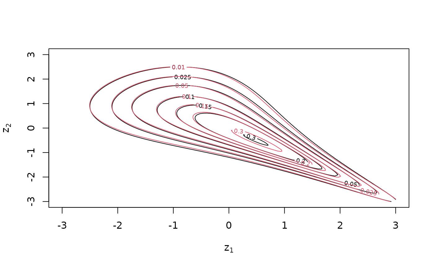
## compare fit with true model
contour(fit)
contour(bicop_dist("clayton", 90, 3), col = 2, add = TRUE)


## fit a model from discrete data
x_disc <- qpois(u, 1)  # transform to Poisson margins
plot(x_disc)

udisc <- cbind(ppois(x_disc, 1), ppois(x_disc - 1, 1))
fit_disc <- bicop(udisc, var_types = c("d", "d"))
summary(fit_disc)
#> Bivariate copula fit ('bicop'): family = gumbel, rotation = 270, parameters = 2.15, var_types = d,d
#> nobs = 100   logLik = 25.96   npars = 1   AIC = -49.93   BIC = -47.32