Plotting tools for bicop_dist and bicop objects

There are several options for plotting bicop_dist objects. The density of a bivariate copula density can be visualized as surface/perspective or contour plot. Optionally, the density can be coupled with standard normal margins (default for contour plots).

Usage

# S3 method for class 'bicop_dist'
plot(x, type = "surface", margins, size, ...)

# S3 method for class 'bicop'
plot(x, type = "surface", margins, size, ...)

# S3 method for class 'bicop_dist'
contour(x, margins = "norm", size = 100L, ...)

# S3 method for class 'bicop'
contour(x, margins = "norm", size = 100L, ...)

Arguments

x

bicop_dist object.

type

plot type; either "surface" or "contour".

margins

options are: "unif" for the original copula density, "norm" for the transformed density with standard normal margins, "exp" with standard exponential margins, and "flexp" with flipped exponential margins. Default is "norm" for type = "contour", and "unif" for type = "surface".

size

integer; the plot is based on values on a size x size grid, default is 100.

...

optional arguments passed to graphics::contour() or lattice::wireframe().

See also

bicop_dist(), graphics::contour(), lattice::wireframe()

Examples

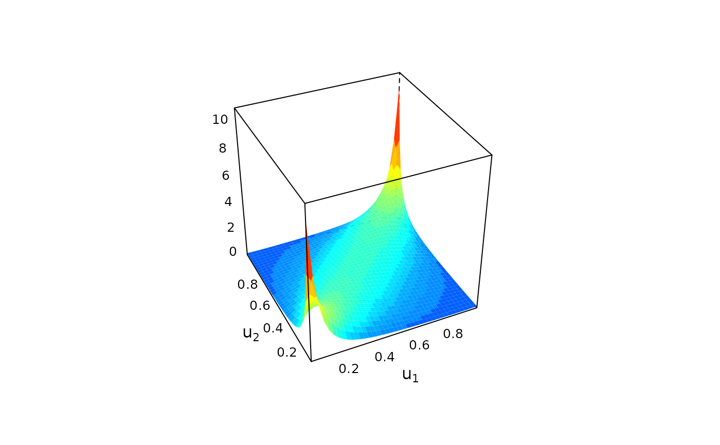
## construct bicop_dist object for a student t copula
obj <- bicop_dist(family = "t", rotation = 0, parameters = c(0.7, 4))

## plots
plot(obj) # surface plot of copula density

contour(obj) # contour plot with standard normal margins

contour(obj, margins = "unif") # contour plot of copula density